In this lecture, t∈R+ denotes the time and we will always assume we have a risky stock.
Definition 1.1 (Stock price):St∈R+ denotes the stock price at time t of the stock S.
Also, we have a “risk-free” bond with continuously compounded interest rate r∈R+.
Definition 1.2 (Bond price):Bt∈R+ is the zero bond price at time t of the bond B.
1.2 Basic Equity Products
An equity derivative is a financial instrument whose value is at least partly derived from one or more underlying equity securities.
Note (max and min notation): We use the notation (⋅)+=max(0,⋅) and (⋅)−=min(0,⋅).
1.2.1 Forwards
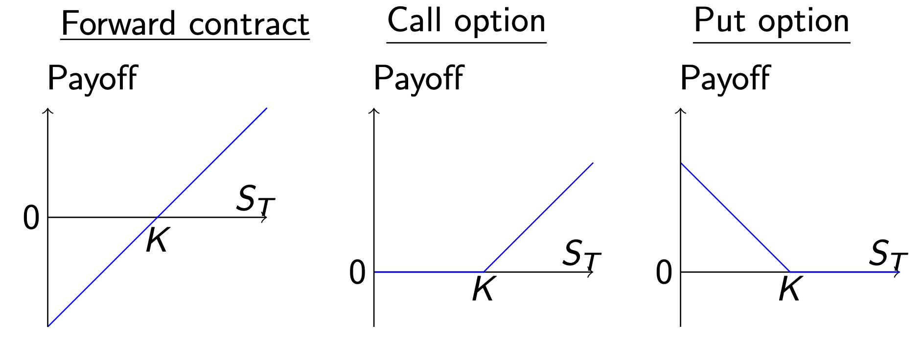
Definition 1.3 (Forward contract): A forward contract F on the stock S is an obligation to buy this stock for a predetermined price K∈R+ at some fixed time in the future T>0 called maturity.
The forward price K remains the same whatever happens to the price of the stock before maturity. The payoff of a forward is F(T,ST,K)=ST−K.
1.2.2 Options
Definition 1.4 (European call option): A European call option C on the stock S is a contract which give the holder of the option the right but not the obligation to buy a stock at a fixed time in the future T>0 called exercise time or maturity for a fixed price K called strike price.
It is clear that the payoff of a call option is C(T,ST,K)=(ST−K)+=max(0,ST−K) because if at time T the stock price ST lies below the strike price K one simply does not execute the call.
Definition 1.5 (European put option): A European put option P on the stock S is a contract which gives the holder of the option the right but not the obligation to sell the stock at a fixed time in the future T for a fixed price K.
Similarly to the call option, it is clear that the payoff of a put option is P(T,ST,K)=(K−ST)+=max(0,K−ST) because if at time T the stock price ST lies above the strike price K one simply does not execute the put.
Figure 1.1: Payoffs at maturity T of a forward contract, a European call option and a European put option with the same strike K.
Note (A word on notation): Sometimes we just write Ct,C(St,K) or C(St) for the payoff C(T,ST,K) depending on the context.
Definition 1.6 (American option): An American call/put option on the stock S is a contract which give the holder of the option the right but not the obligation to buy/sell the stock at any point in time in the future up to maturity T for a fixed price K.
Note (Contingent claim): A contingent claim is a financial contract whose payoff depends on the future value of some underlying asset or assets. The key characteristic is that the payment or settlement is “contingent” on, i.e. depends on, how certain events unfold in the future. Futures and options are examples for contingent claims.
1.3 No Arbitrage Pricing
We note that a financial derivative is defined in terms of some underlying asset whose price one sees in the market. Hence, the derivative cannot be priced arbitrarily. There exists an intimate relation between the price of the underlying and the derivative. Neglecting this relation gives rise to mispricing.
The theory of derivatives is about pricing relative to the market price of the underlying. It is not concerned about pricing in absolute terms.
1.3.1 Assumptions
All derivative pricing models are based on the no arbitrage assumption.
Definition 1.7 (No arbitrage assumption): It is not possible to build a portfolio π such that at time t=0 the value is zero, i.e. V0(π)=0, and the value at some time in the future T>0 can be positive, i.e. P(VT(π)>0)>0, but not negative, i.e. P(VT(π)≥0)=1.
Example (Arbitrage): Assume that we have two stocks, S(1) and S(2). At time t=0 both stocks are priced equally at S0(1)=S0(2)=10 and we short one stock S(1) and buy one stock S(2) s.t. our portfolio value is V0(π)=(−1)⋅S0(1)+(1)⋅S0(2)=0. Lets assume that at time t=1 the stock prices can either go both up, i.e. S1(1)=S1(2)=15 with probability pu, or both down, i.e. S1(1)=5 and =S1(2)=5.1. In case of a price increase our portfolio value stays at V1(π)=(−1)⋅S1(1)+1⋅S1(2)=0. In case of price decrease we have V1(π)=(−1)⋅S1(1)+1⋅S1(2)=0.1. Hence we have arbitrage as P(V1(π)>0)>0 and P(V0(π)≥0)=1.
Furthermore, we will always assume no market frictions.
Definition 1.8 (No market frictions assumption): We assume the following:
We can buy/sell any fraction of shares.
We can buy/sell unlimited amounts of shares.
There is no bid/ask spread.
There are no transaction costs.
There are no taxes.
A market is arbitrage free if there is no arbitrage portfolio.
Definition 1.9 (Law of One Price): If two portfolios π1 and π2 have the same value VT(π1)=VT(π2) at some time in the future T>0, then ∀t≤T we have Vt(π1)=Vt(π2).
Proposition 1.10 (No arbitrage implies Law of One Price): A market without arbitrage opportunity satisfies the Law of One Price.
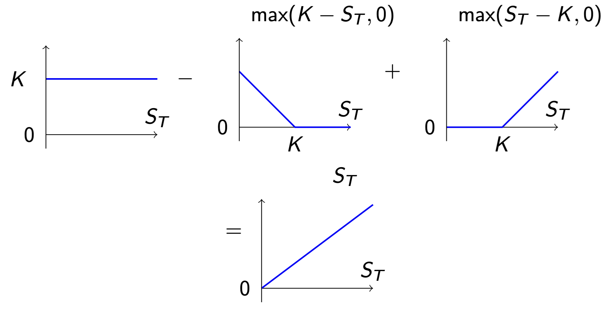
Example (Put-call parity): Lets assume the portfolios π1 where we long K bonds and one call and short one put, i.e. Vt(π1)=KBt−Pt+Ct, and π2 where we long the underlying share, i.e. Vt(π2)=St. At maturity of options and bond at some time T in the future we have
VT(π1)=K−max(K−ST,0)+max(ST−K,0)=ST=VT(π2)
Therefore, under the Law of One Price, π1 and π2 have the same value at all times, i.e. KBt−Pt+Ct=St.
Figure 1.2: The portfolios π1 and π2.
Example (Fair strike of a forward): We want to find out fair price, i.e. the arbitrage free, strike price K of a forward contract F with maturity T. Lets assume we F. At time t=0 we buy the underlying stock for price S0 such that we are able to sell it at time T. As this contract should have no cost we borrow S0 from the bank. At time T we receive K for the stock and have to reimburse the bank S0erT, hence we cover our debts exactly when K=S0erT.
1.4 Static and Dynamic Replication
In the following, let π and π~ be portfolios.
Definition 1.11 (Replication): Replication is the process of finding the value of the portfolio π at time t by building another portfolio π~ s.t. VT(π)=VT(π~) at some point in the future T. By the Law of One Price we have ∀t≤T:Vt(π)=Vt(π~).
Definition 1.12 (Static replication): We build our portfolio π~ without rebalancing s.t. VT(π)=VT(π~).π~ is called a static replicating portfolio.
Example (Convertible bond valuation): TODO
Note (Properties of static replication): Because of the lack of rebalancing, static replication is model independent as no probability assumptions have to be made. We also note that in practice it is generally not possible to find a static replication portfolio as the efficient market assumption does not hold and constant rebalancing is needed.
Definition 1.13 (Dynamic replication): We build our portfolio π~ and we readjust it at any time needed s.t. VT(π)=VT(π~).π~ is called a dynamic replicating portfolio.
Note (Properties of dynamic replication): As we allow for rebalancing, we now have to make probabilistic assumptions for the evolution of π~. We note that in complete, but not necessarily efficient, markets it is possible to find a dynamic replicating portfolio.
Examples for dynamic replications are the Binomial model, the Black-Scholes model and its extensions.