We are motivated by the fact that no static replicating portfolio of European options and other products exists. We thus have to develop a dynamic replicating portfolio based on an appropriate model.
2.1 One-Period Binomial Model
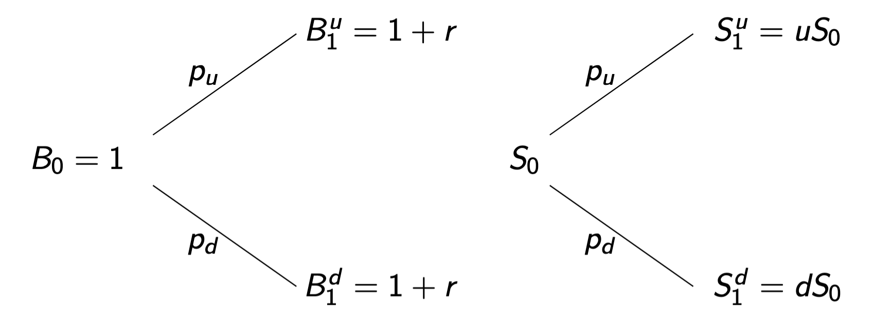
Our market consists of two basic instruments, a stock S and bond B, with a starting state at t=0 and two possible states at t=1.
Figure 2.1: The market at time t=0 and t=1.
We call the measure P with the probabilities pd and pu the historical measure and impose the following requirements:
non-negative stock price: S0>0
lower bound on interest rate: r>−1
positive, ordered stock price movements: u>d>0
non-zero probabilities: 0<pd,pu<1
Definition 2.1 (Portfolio in one-period binomial model): The value πt=xSt+yBt of a portfolio π is composed of x∈R units of stock S and y∈R units of bond B.
As
t \in \cb{0,1}
we only have to consider π0=xS0+yB0 and π1=xS1+yB1.
Definition 2.2 (Arbitrage portfolio for the one-period model):π is an arbitrage portfolio if and only if π0=0 and π1≥0 with a positive probability of making profits P(π1>0)>0.
Hence an arbitrage portfolio is a strategy where you can make money out of nothing. We aim at building models that are arbitrage-free and search for so called NA, i.e. no-arbitrage, conditions for the model parameters to ensure this.
Definition 2.3 (NA condition for one-period binomial model): The one-period binomial model has no arbitrage if and only if 0<d<1+r<u.
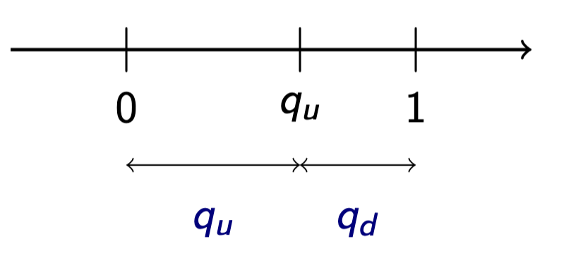
As NA implies 1+r∈(d,u) we can write 1+r as a convex combination of d and
u, i.e. 1+r=qdd+quu where
qu=u−d(1+r)−dandqd=u−du−(1+r)
and qu+qd=1.
Figure 2.2: Illustration of qu and qd.
We can interpret
\cb{q_u, q_d}
as a new probability measure
Definition 2.4 (Risk-neutral measure): The artificial measure Q with the probabilities
In other words, the discounted expectation under the risk-neutral measure of the stock price tomorrow is equal to the stock price today.
Recall that a process (Xt)t≥0 is a martingale under a probability measure μ if
\E_{\mu}[X_{t+1} \mid X_t] = X_t
, i.e. if the estimated value for the future value at t+1 is its current value Xt.
Example (Discounted stock price): Take Xt=(1+r)tSt and the risk neutral measure Q. We know that
\E_{\Q}\bk{\frac{1}{1+r} S_1 \mid S_0} = S_0
i.e. the discounted stock price is a martingale under the risk-neutral measure for the one-period binomial tree.
Definition 2.5 (Martingale measure): The probability measure Q is a martingale measure w.r.t. the discounted stock price if and only if
\E_{\Q}\bk{\frac{1}{1+r} S_1 \mid S_0} = S_0
.
Note (Equivalent measures): We call two measure μ,ν equivalent if for all events ω∈Ω we have μ(ω)=0⟺ν(ω)=0.
Theorem 2.6 (First fundamental theorem of asset pricing): The NA condition holds if and only if there exists a martingale measure Q equivalent to the historical measure P.
Martingale measures are extremely useful as their existence guarantees NA and they will give us the no-arbitrage price of any asset.
Recall that our aim is to price options. We provide an example of a dynamic replication in the context of the one-period binomial model.
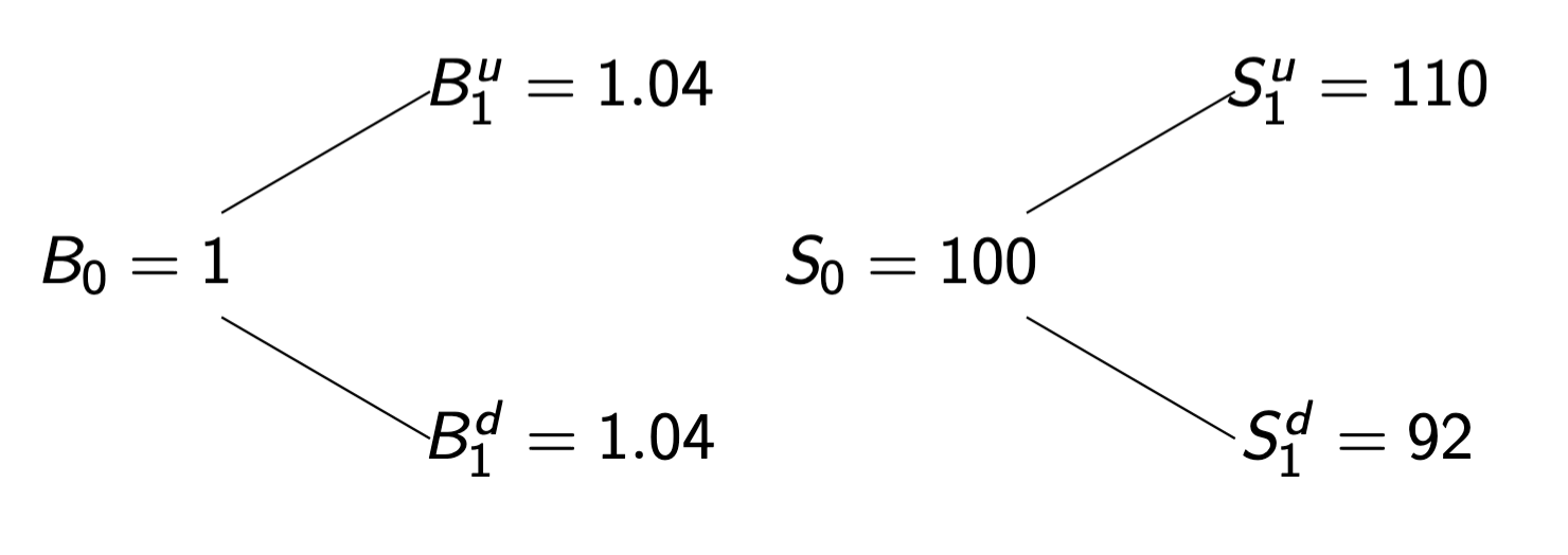
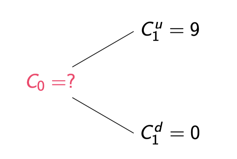
Example (Pricing European options): Consider a European call option on a stock S with maturity T=1 and strike K=101. Let S0=100,r=4%,u=1.1 and d=0.92.Figure 2.3: The possible states at time t=0 and t=1.At maturity, the payoff is C1=(S1−K)+, thus we have C1u=(S1u−K)+=9 and C1d=(S1d−K)+=0.Figure 2.4: The option values at time t=0 and t=1.We replicate the option using the underlying assets at disposal, i.e. we consider a portfolio π composed of α stocks and β bonds, s.t. πt is characterized by
π1u=110α+1.04β=9=C1uπ1d=92α+1.04β=0=C1d
Solving the linear equations entails β=−1.0446≈−44.23 and α=21. Hence πt=21St−1.0446Bt replicates the option Ct and because of the Law of One Price this is true independently of t. Thus we receive C0=π0=21S0+1.0446B0≈5.77 as the fair value of the option at time t=0.
2.1.1 Completeness
Definition 2.7 (Complete model): A model is considered complete when every contingent claim can be perfectly replicated using only the underlying asset S and the risk-free asset B.
In other words, completeness ensures that for any derivative security with a given payoff K at maturity, we can construct a self-financing portfolio that exactly matches K using only the two basic instruments B and S.
Proposition 2.8 (Completeness of the one-period binomial model): The one-period binomial model is complete as there are at least two assets for two possible future states and the two assets are linearly independent.
Completeness is an attractive feature because we get a hedging portfolio for each contingent claim. However, it also means that contingent claims are superfluous since we can trade in the stock/bond and replicate it.
In practice the market is not complete, i.e., it is not possible to hedge any contingent claim only trading a risk-free bond and the stock. The model is overly simplistic.
2.1.2 Martingale Pricing
We summarize the aforementioned results.
Proposition 2.9 (Martingale pricing in the one-period binomial model): In the one-period binomial model, no arbitrage implies that the price H0 of any contingent claim H1 given by
H_0=\frac{1}{1+r} \E_{\Q}\bk{H_1}
where Q∼P is the martingale measure given by qu=u−d(1+r)−d,qd=u−du−(1+r).
In other words, under a martingale measure, the price of any contingent claim is given by the expectation of its discounted payoff. Hence, this theorem allows to price a contingent claim without dealing with replication.
Theorem 2.10: In the absence of arbitrage, the market is complete if and only if there exists a unique equivalent martingale measure Q.
This allows to link replication and completeness to the martingale measure. It is often easier to work with martingale measures than with portfolios.
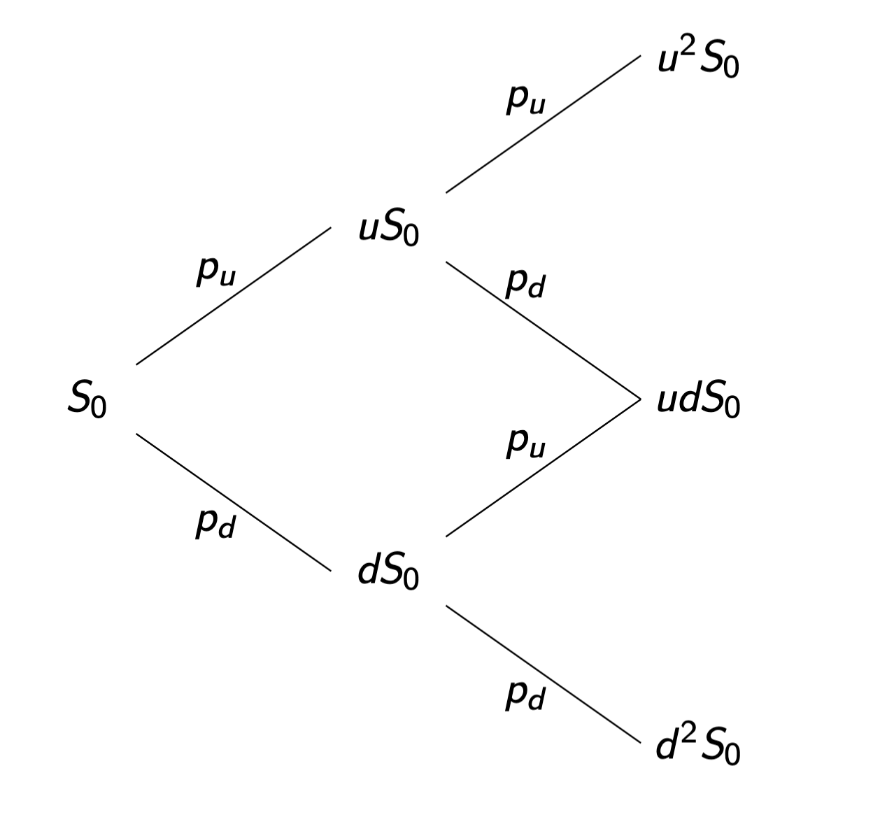
2.2 Multiperiod Binomial Model
The multiperiod binomial model improves upon the one-period model. From t0=0 to t=T it allows more than one move of the underlying stock S and more than two states in the economy. We achieve this by increasing the number of periods in the binomial model.
Figure 2.5: The first two timesteps of the multiperiod binomial model.
We divide our period of interest [0,T] into N equal-length periods
\bk{t_k, t_{k+1}}
, with tk=NkT for 0≤k≤N. At each time tk we hace the two assets with prices Bk and Sk.
To calculate the bond price in the multiperiod binomial model, we assume that the annual interest on the bond is r. Hence the one-period interest rate is r~=rNT assuming that T is measured in years. Thus Bk+1=(1+r~)Bk. Note that when N→∞, we have limN→∞BN=limN→∞(1+r/TN)N=erT through continuous compounding.
Note that the stock price is set to Sk at time t∈[tk,tk+1), i.e. the function of stock prices over time is step-wise.
2.2.1 Stock Distributional Properties
The probabilistic evolution of the stock does not depend on its past, only on its present, i.e. P(Sk+1∣S0,…,Sk)=P(Sk+1∣Sk).
We derive the distribution of the stock price by induction. At time t1,S1 can take 1+1 values: uS0 and dS0 with probabilities P(S1u)=pu and P(S1d)=pd respectively. Hence at time tN=T,SN can take N+1 values: uidN−iS0,∀0≤i≤N with probabilities
P(SN=S0uidN−i)=(iN)puipdN−i
respectively.
2.2.2 Trading Strategy
Under the context of the multimodal binomial model we refine the definiton of a portfolio/trading strategy.
Definition 2.11 (Trading strategy): A trading strategy/portfolio strategy πt is a discrete time stochastic process that is composed of xk∈R units of stock S and yk∈R units of bond B at time tk. We are only allowed to change our portfolio just after the stock price has moved, i.e. at times tk+, thus πt=(xt,yt)=(xk,yk) for t∈(k−1,k).xk and yk are only allowed to depend on S0,…,Sk−1. The value of the portfolio is therefore
πt={πk=xkSk+ykBkπk+=xk+1Sk+yk+1Bkfor t=tkfor t∈(tk,tk+1)
We are interested in strategies where we do not need to inject/remove capital.
Definition 2.12 (Self-financing trading strategy): A trading strategy is self-financing if we have xkSk+ykBk=πk=πk+=xk+1Sk+yk+1Bk for all k=0,…,N−1.
In other words, when rebalancing our portfolio
\cb{x_k, y_k} \rightarrow \cb{x_{k+1}, y_{k+1}}
, the value of our portfolio does not change. The value of the portfolio can only change due to movements in the assets B and S.
2.2.3 No Arbitrage
We extend the definition of the arbitrage portfolio to the multiperiod model.
Definition 2.13 (Arbitrage portfolio): A self-financing trading strategy π is an arbitrage if and only if V0=0,P(VN≥0) and P(VN>0)>0.
Definition 2.14 (NA condition in the multiperiod binomial model): The following statements are equivalent:
There is no arbitrage in the multiperiod binomial model
There is no arbitrage in each one-period sub model
We have 0<d<1+r~<u
Thus the N-period model has the same non arbitrage condition and properties as the one-period model. We can therefore define the martingale measure in the multiperiod model.
Definition 2.15 (Martingale measure in the multiperiod binomial model): A martingale measure or risk-netral measure is a probability measure Q such that
In other words, a measure Q is a martingale measure in the N-period model if and only if it is a martingale measure for each sub-period model.
From the one period model we therefore know that NA implies the existence of an equivalent martingale measure Q, that qu=u−d(1+r~)−d,qd=u−du−(1+r~) define such measure and that the measure is unique.
We extend the market completeness property to the general binomial model.
Theorem 2.16 (Market completeness for the binomial model): The binomial model is complete. In particular, let VN be the payoff of a simple European security and define
, the value of the self-financing portfolio process α0,…,αN−1 is the process V1,…,VN.TODO
In other words, market completeness implies that e.g. a simple European security can always be hedged.
2.2.4 Binomial Option Pricing Formula
Definition 2.17 (Binomial algorithm): Under no-arbitrage, the price Hki at time tk of any contingent claim H with payoff HN=H(SN) at time T is given by the following algorithm
At time tN there are N+1 nodes defined e.g. by the number of times i the stock goes up. There are
\# \qty{S_N = u^i d^{N-i} S_0} = \binom{N}{i}
paths leading to this node. All paths are independent of each other and have risk-neutral probability quiqdN−i, hence
Q(SN=uidN−iS0)=(iN)quiqdN−i
We can thus formulate the binomial option pricing formula.
Definition 2.18: The price at time t=0 of a European contigent claim H with payoff H(SN) at time T is given in the multiperiod binomial model by the binomial option pricing formula
H0=(1+r~)N1i=0∑N(iN)quiqdN−iH(S0uidN−i)
2.2.5 Rewriting the Call Option Formula
We consider now a European call option with maturity after N timesteps. For the claim to be exercisable, we require the option to be in the money, i.e. S0ujdN−j>K. Hence, we can determine the minimal number of up-moves for the underlying as
A=⌊ln(u/d)ln(K/(S0dN))⌋+1
For simplification we write 1+r~=R. Then, we can rewrite the formula for the call option as
where q′=Rqu and Ψ(a,n,p) is the complimentary binomial distribution function. More specifically, Ψ(a,n,p) describes the probability of getting at least a heads out of n tosses if the probability for heads is p.
Recall that we have defined our timestep delta to be h=NT. One can show that in the limit h→0, i.e. N→∞, the aforementioned rewritten call option formula converges to
C0=S0N(d1)−Ke−rTN(d2)TODO where N is the standard normal density function and