In this section we assume that the SCLM holds. We start by recapping some important distributions.
Recap (Chi-squared distribution): Let Z1,…,Zd∼iidN(0,1). Then U=∑i=1dZi∼χd2. We have E[U]=k and Var[U]=2k.
Recap (T distribution): Let Z∼N(0,1) and U∼χd2 be independent. Then T=d−1UZ∼td. We have E[T]=0. For d>2, we have Var[T]=d−2d.
Recap (F distribution): Let U∼χd12 and V∼χd22 be independent. Then F=d2−1U2d1−1U1∼Fd1,d2. For d2>2 we have E[F]=d2−2d2. For d2>4 we have Var[F]=d1(d2−2)2(d2−4)2d22(d1+d2−2).
Note: If T∼td then T2=Ud−1Z2∼F1,d.
4.1 Basic Test Statistics
We first assume that σ2 is known. We know that β^∼N(β,σ2(X⊤X)−1). We want to test the null hypothesis H0:βj=0. We can then construct a two-sided test. We do that by noting that under null hypothesis we have
T=σ(X⊤X)[j,j]−1β^j∼N(0,1)
This is our test statistic. We can then compute the p-value of the observed test statistic by p=P(∣T∣>∣t∣)=2Φ(−∣t∣) and compare it to a pre-determined test significance level α∈[0,1]. We reject H0 if p≤α.
4.2 Basic Confidence Interval
Note: Given a random variable X, we use σX=Var[X] to denote the standard deviation and σ^X to denote a suitable estimator. σ^X is often called standard error in the literature.
We assume the same setting as before and want to find a (1−α) confidence interval for βj. As the standard Gaussian is symmetric we have
σ(X⊤X)[j,j]−1βj−β^j∼N(0,1)
and thus the confidence interval
P(β∈[β^j−σβ^jz1−21α,β^j+σβ^jz1−21α])=1−α
where z1−21α=Φ−1(1−21α).
Note: The (1−α) confidence interval is equivalent to the set of all parameter values that would not be rejected by the hypothesis test for H0 at significance level α.
4.3 Test and CI Distributions
We assume now that σ2 is not known. We can construct the following distributions for test statistics and confidence intervals.
Proposition 4.1 (Individual parameter): For each parameter βj we have
σ^β^jβ^j−βj∼tn−p
where σ^β^j=σ^(X⊤X)[j,j]−1.
Proof: TODO
We can use the t-test statistic T=σ^β^j−1β^j to test whether the coefficient βj is significantly different from zero.
Proposition 4.2 (Entire parameter vector): For the entire parameter vector β we have
pσ^2X(β^−β)2=pσ^21(β^−β)⊤X⊤X(β^−β)∼Fp,n−p
Proof: TODO
We can use the zero-model F-test statistic T=(pσ^2)−1∑i=1nY^i2 to test whether the entire parameter vector β is significantly different from the zero vector 0. We discuss the F-test in detail in the next section.
Proposition 4.3 (Subset of parameter vector): For a subset or linear transformation b=Bβ with B∈Rr×p and rank(B)=r we have
pσ^21(b^−b)V−1(b^−b)∼Fq,n−p
where V=B(X⊤X)−1B⊤.
Proof: TODO
As discussed in the next section, we use B=[I0] to define a partial F-test.
Proposition 4.4 (Expectation of observation): For the expectation of the i-th observation Yi, that is E[Yi]=β⊤xi, we have
σ^Y^iY^i−E[Yi]∼tn−p
where σ^Y^i=σ^P[i,i].
Proof: TODO
Note: It is important to note that we target the true value, i.e. the expected value E[Yi], and not the observation Yi itself.
Proposition 4.5 (Expectation of observation under any condition): For the expectation of an observation Yn+1 under an arbitrary experimental condition xn+1, that is E[Yn+1]=β⊤xn+1, we have
σ^Y^n+1Y^n+1−E[Yn+1]∼tn−p
where σ^Y^n+1=σ^xn+1⊤(X⊤X)−1xn+1.
Proof: TODO
Note: We again target the expected value E[Yi]. In the case that xn+1=xi for some i∈{1,…,n} we have xi⊤(X⊤X)−1xi=P[i,i] and σ^Y^n+1=σ^Y^i.
Proposition 4.6 (New observation): For a new observation Yn+1 under the experimental condition xn+1, we have
σ^Y^n+1−Yn+1Y^n+1−Yn+1∼tn−p
where σ^Y^n+1−Yn+1=σ^1+xn+1⊤(X⊤X)−1xn+1.
Proof: TODO
Note: Here we target the observation Yi itself thus introducing new variability to the distribution.
4.4 F-test and its Geometric Interpretation
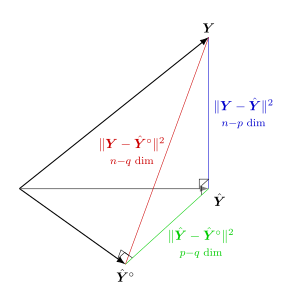
Recall that we assume SCLM, thus the linear model Y=Xβ+ε is correct. Let H0 be the hypothesis H0:βq+1=0,…,βp=0, i.e. only the first q coefficients are non-zero. We construct the nested model by defining the n×q submatrix X∘=X[:,1,q] and the subvector β∘=(β1,…,βq). Then, under H0,X∘ and β∘ would suffice to define Y, i.e. Y=X∘β∘+ε. The following orthogonality holds regardless of H0.
Proof: As Y^=PY, we know that (Y−Y^)⊥R(X). We note that R(X∘)={z∈Rn∣z=X∘b}⊆R(X). As Y^∘∈R(X∘), we have (Y^−Y^∘)∈R(X). Therefore, (Y−Y^)⊥(Y^−Y^∘).
Note: The name nested model comes from the fact that R(X∘)⊆R(X).
Applying Pythagoras, this leads to the following decompositon of the residual sum of squares or RSS.
Figure 4.1: RSS decomposition given a nested model.
We summarize what we know about the RSS components:
Under SCLM, σ21ε^⊤ε^=σ21Y−Y^2∼χn−p2
Under SCLM, (Y−Y^) and (Y^−Y^∘) are independent as they are orthogonal and ε is idiosyncratic
Under H0,σ21ε^∘⊤ε^∘=σ21Y−Y^∘2∼χn−q2
Thus, under H0, as Y^−Y^∘2=Y−Y^∘2−Y−Y^2, we have σ21Y^−Y^∘2∼χp−q2
Hence, we can construct the test statistic for the partial F-test as follows
T=(n−p)−1Y−Y^2(p−q)−1Y^−Y^∘2∼Fp−q,n−p
Note:
The partial F-test statistic has the relationship tan(δ)2∝T where δ=∠(Y^−Y^∘,Y−Y^). The bigger the statistic, the bigger the angle δ and the more unlikely it is that the nested model and thus H0 is true.
In other words, we test whether Y^−Y^∘ is significantly longer than what random noise would produce by comparing it to one “unit” of random variance σ^2=(n−p)−1Y−Y^2.
It can be shown that the partial F-test statistic can be equivalently derived by using the distribution for the subset of a parameter vector with the (p−q)×p transformation B=[0I] and H0:b=0.
It can happen that Ha,0:β1=0 and Hb,0:β2=0 are not rejected but Hc,0:β1=β2=0 is rejected. This means that the covariates x:,1 and x:,2 are heavily correlated and either one can be left out but not both.
The zero-model F-test statistic emerges from the nested model with q=0, i.e.
T=(n−p)−1ε^⊤ε^p−1Y^2=(pσ^2)−1i=1∑nY^i2
However, the zero-model baseline H0:β=0 is almost always trivially significant because the response variable's averge is rarely zero. A better baseline is discussed in the next section.
4.5 Coefficient of Determination
Usually, we use the location model Yi=β+εi as the reference nested model, as it provides a simple baseline corresponding to Y^=Y.
Proposition 4.9 (Global F-test): The global F-test statistic F compares the full model to the nested model with just the intercept, i.e.
F=(n−p)−1Y−Y^2(p−1)−1Y^−Y2∼Fp−1,n−p
It tests the hypothesis H0:β2=0,…,βp=0.
Note: The partial F-test statistic can be equivalently dervide by using the distribution for the subset of a parameter vector with the (p−1)×p transformation B=[0I] and H0:b=0.
One important quantity is the coefficient of determination.
Definition 4.10 (Coefficient of determination): The coefficient of determination is
R2=z∈R(X)maxcor(Y,z)2
Proposition 4.11 (Intercept case): If the full model has an intercept, the coefficient of determination is
R2=Y−Y2Y^−Y2
Proof: TODO
Note: In the following we assume the full model has an intercept:
R2 is the proportion of variance explained by the full model compared to the total variance.